
Chi-Squared testing
Null hypothesis: The proportion of people who choose the same hotel again will be the same for beach combers and windsurfers.
To start off, I constructed my data.frame in a very roundabout manner:
>Beachcomber <- c(163,64,227)
>Windsurfer <- c(154,108,262)
>Choose_again <- c("Yes", "No", "Total")
>dat <- data.frame(Choose_again, Beachcomber, Windsurfer)
>dat$Total <- dat$Beachcomber + dat$Windsurfer
>dat <- dat[,-1]
>rownames(dat) <- c("Yes", "no","total")

>dat

      Beachcomber Windsurfer Total
Yes           163        154   317
no             64        108   172
total         227        262   489
Next, I run the chi-test and save it in an object:
>res<-chisq.test(dat[1:2,1:2])
> res

Pearson's Chi-squared test with Yates' continuity correction

data: dat[1:2, 1:2]
X-squared = 8.4903, df = 1, p-value = 0.0035
I was stuck on that for a while, trying to figure out exactly which parts of the data.frame needed to be included/excluded. I did notice that this way of doing it didn’t give me the error that other combinations did though. I assume it’s because the function implemented Yates’ continuity correction, which is automatically implemented for 2×2 tables. The p-value is quite small, so at a threshold of p=.05, the null hypothesis would be rejected and we’d say that it appears that the proportion of people who choose to return to their hotel is different for each group.
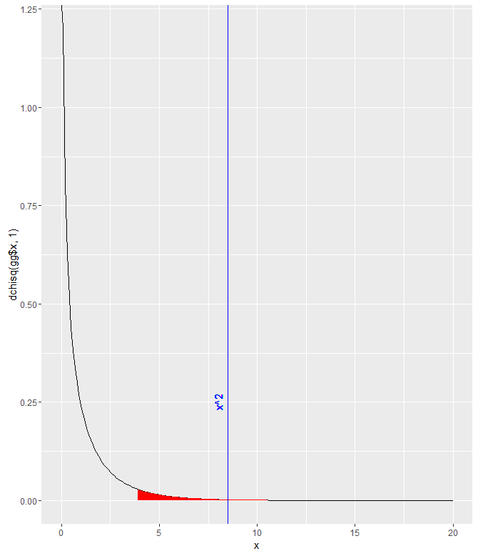
gg <- data.frame(x = seq(0,20,.1))
gg$y <- dchisq(gg$x, 1)
ggplot(gg) +
 geom_path(aes(x,y)) +
 geom_ribbon(data=gg[gg$x>qchisq(.05,1,lower.tail=FALSE),], aes(x,ymin=0, ymax=y), fill="red")+
 geom_vline(xintercept = res$statistic, color = "blue")+
 labs( x = "x", y = "dchisq(gg$x, 1)")+
 geom_text(aes(x=8, label="x^2", y=0.25), colour="blue", angle=90)