
An analysis of hashtags on Zika related tweets
I have a set of 359,043 tweets (object named zq) with 27 variables from 8/25 -9/5 that have the word “zika” in them. After removing any tweets that have duplicate tweet_id’s and tweets that are scraped/parsed incorrectly, I was left with 358,613 tweets. I would like to determine how different hash tags effect how often a tweet with an image gets retweeted.
From looking at the data previously, I noticed that bees were a hot topic and not something we normally think about within the context of zika. I suspect that, within the data set, using bees as a hashtag will be associated a higher amount of retweets per tweet than some other tweets. I’m going to compare #bees with #zika and #mosquito.
H0: # of retweets per tweet ( bees = zika = mosquito )
H1: # of retweets per tweet ( bees > zika | mosquito )
To start off, we need to isolate the tweets that have embedded images. I have determined that the easiest and most accurate way to identify an embedded image is to look for “photo/1” in the parsed_media_url field of the data set:
zqimage <- zq[grep("photo/1", zq$parsed_media_url),]
This leaves us with 83,266 tweets that have images embedded in them. Now, the hashtags are stuck within the “hashes” column, and are delimited by semicolons. Using tidyr, we can separate those out into more columns:
library("tidyr")
zq1 <- separate(zqimage, col = hashes, into = c("hash1", "hash2", "hash3",
 "hash4", "hash5", "hash6", "hash7", "hash8", "hash9", "hash10", "hash11",
 "hash12", "hash13", "hash14", "hash15", "hash16", "hash17", "hash18", "hash19",
 "hash20"), sep = ";", extra = "merge", fill = "right")
This adds 19 more columns, which should then either have their own hashtag, or a N/A value. From here, we can use apply to count up the frequency of each hashtag and create a table to show us what the 30 most popular hashtags are:
library("plyr")
hashes <- apply(zq1[,24:43], 2, FUN=function(x) plyr::count(x))
hashes <- do.call(rbind.data.frame, hashes)
hashes <- plyr::ddply(hashes,"x",numcolwise(sum))
hashes <- hashes[!is.na(hashes[,1]),]
hashes <- head(arrange(hashes,desc(freq)), n = 100)
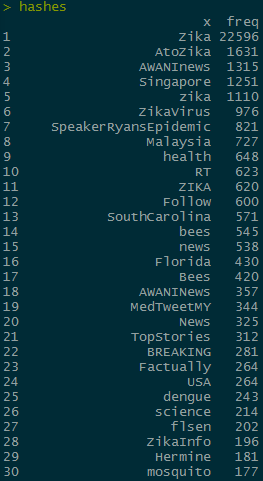
The hashtags I want to compare are “bees” and “mosquito” which are the 14th and 30th most common hashtags, respectively. In order to do further analysis, I need to subset the rows to only include the max value of retweet_count for each unique tweet. I’m going to do it to zqimage instead of the hashes object so that I can use grep on the non separated hashes column later:
library("dplyr")
zqimage <- zq[grep("photo/1", zq$parsed_media_url),]
zqimage <- zqimage %>% group_by(text) %>% filter(retweet_count == max(retweet_count),
 favorite_count == max(favorite_count))
zqimage <- arrange(zqimage, desc(retweet_count))
I want to compare the contributions between hash tags, so I can get rid of any rows that don’t have any hashtags
zqimage <- zqimage[!is.na(zqimage$hashes), ]
This leaves us with 9,651 unique tweets that have hashtags and have embedded images. In order to conduct an ANOVA test we need to categorize the tweets. In order to do so, we need to create a new column that says if the tweets have “bees”, “mosquito”, or “zika” in them
zqimage$hashhash <- ifelse(grepl("bees", zqimage$hashes, ignore.case = TRUE), "bees",
 ifelse(grepl("mosquito", zqimage$hashes, ignore.case = TRUE), "mosquito",
 ifelse(grepl("zika", zqimage$hashes, ignore.case = TRUE), "zika", "Other")))
From here, we can apply the ANOVA test
fit <- aov(zqimage$retweet_count ~ hashhash, data = zqimage)
Making a boxplot of the data shows something very telling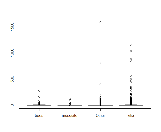
It looks like there’s an oppressive amount of tweets with abnormally high values of retweets that are making it hard to see what’s going on, so lets look at a log scale of only the tweets that have been retweeted.
zqn0 <- zqimage[!zqimage$retweet_count == 0,]
boxplot(log(zqn0$retweet_count) ~ zqn0$hashhash
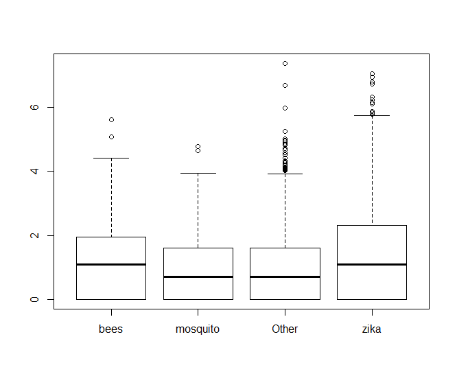
From there, we can see clearly that hashtags with bees performs better than mosquito, but it looks almost neck-and-neck with zika. If we look at the values of fit$coefficients, we can see that bees edges out zika in performance too.
> fit$coefficients
 (Intercept) hashhashmosquito hashhashOther hashhashzika
  7.1780822        -4.9327290    -4.8003600   -0.9336632
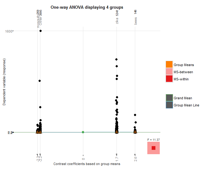
I used the granovagg package to create the above graphic which again shows that bees outperforms mosquito, even though mosquito had nearly an order of magnitude fewer hashtags than case-insensitive “bees”, and it also outperforms case-insensitive “zika” despite the fact that zika hashtags had over 22,000 more hashtags.
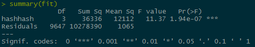
The p value for the hashes is very small, causing us to fail to reject the null hypothesis and accept the alternate hypothesis that the bees hashtags perform better than the mosquito or zika hash tags.