by Ryan | Apr 4, 2016 | intro to r programming
The process of setting up git with RStudio was not as straight-forward as I had expected. I had not realized that git was different from the Github desktop app. Trying to tie the Github desktop app into R Studio caused R Studio to keep opening up new instances of the Github desktop app while it tried to establish a connection to the website. After realizing that there was, in fact, a difference between git and the desktop app, I refocused my efforts on git. After redoing all the configuration, I tried to push my package to github only for it to fail again. Somewhere along the line of my configurations, the actual repository itself didn’t get created.
For the package itself, I tried to make a simple series of functions to do some goat census work for a game I play. It didn’t go well at all. I’m currently taking java, so I’m having some challenges switching back and forth between syntaxes, causing some turbulence with creating some simple loops. I spent an embarrassing amount of time trying to figure out why my loop wasn’t working (I do know that loops aren’t common in R). It turns out that ++i doesn’t work. In the midst of me trying to work that out, I was trying to have my functions stand alone in their own files to be called from the main file, and that wasn’t working at all either. I tried various source declarations and, in the end, wasn’t able to get it to work. All of this troubleshooting left me with a sad little shriveled raisin of a package.
by Ryan | Mar 29, 2016 | intro to r programming
For this exercise, I again used the sleep study data from https://vincentarelbundock.github.io/Rdatasets/csv/lme4/sleepstudy.csv. I assigned the values for the numbers of days and the reaction times to the x and y values to matrix ‘x’. Next, I created the function for tukey.multiple().
> tukey_multiple <- function(x) {
+ outliers <- array(TRUE,dim=dim(x))
+ for (j in 1:ncol(x))
+ {
+ outliers[,j] <- outliers[,j] && tukey.outlier(x[,j])
+ }
+ outlier.vec <- vector(length=nrow(x))
+ for (i in 1:nrow(x))
+ {
+ outlier.vec[i] <- all(outliers[i,])
+ }
+ return(outlier.vec)
+ }
To start debug mode, you must first initialize it with > debug(tukey_multiple) and then try executing the function itself with > tukey_multiple(x). The debug mode spits out an error saying that it can’t find the function tukey.outlier, which is called for in line 5. In order to find the outliers we must first be able to identify why is and is not an outlier. In order to do so, we have to make a function to define the quartiles in the set of data:
> quartiles = function(data)
+ {
+ quarts = quantile(data, probs=c(.25,.75))
+ IQR = quarts[2] - quarts[1]
+ return(c(quarts,IQR))
+ }
Now that we have the quartiles, we can make a function to pull out the outliers:
>tukey.outlier = function(q)
+ {
+ if(!is.nutll(dim(q))){
+ return(tukey_multiple(q))
+ } else {
+ quarts = quartiles(q)
+ lowerbound = quarts[1] - 1.5*quarts[3]
+ upperbound = quarts[2] + 1.5*quarts[3]
+ outliers = c(rep(FALSE, length(q)))
+ outliers <- ((q < lowerbound) | (q > upperbound))
+ return(outliers)}
+ }
Moving forward from here, we can try to run >tukey_multiple(x) again. Doing so gives me an error “Error in tukey.outlier(x[, j]) : could not find function “is.nutll””. This one is due to a simple typo of is.null. This is fixed and the debug for tukey_multiple is ran again. The debug makes it past the previous errors and I proceeded through hitting enter through all 180 values of my data, ending in this:
exiting from: tukey_multiple(x)
 [1] FALSE FALSE FALSE FALSE FALSE FALSE FALSE FALSE FALSE FALSE FALSE FALSE FALSE FALSE FALSE FALSE FALSE FALSE FALSE FALSE FALSE FALSE
 [23] FALSE FALSE FALSE FALSE FALSE FALSE FALSE FALSE FALSE FALSE FALSE FALSE FALSE FALSE FALSE FALSE FALSE FALSE FALSE FALSE FALSE FALSE
 [45] FALSE FALSE FALSE FALSE FALSE FALSE FALSE FALSE FALSE FALSE FALSE FALSE FALSE FALSE FALSE FALSE FALSE FALSE FALSE FALSE FALSE FALSE
 [67] FALSE FALSE FALSE FALSE FALSE FALSE FALSE FALSE FALSE FALSE FALSE FALSE FALSE FALSE FALSE FALSE FALSE FALSE FALSE FALSE FALSE FALSE
 [89] FALSE FALSE FALSE FALSE FALSE FALSE FALSE FALSE FALSE FALSE FALSE FALSE FALSE FALSE FALSE FALSE FALSE FALSE FALSE FALSE FALSE FALSE
[111] FALSE FALSE FALSE FALSE FALSE FALSE FALSE FALSE FALSE FALSE FALSE FALSE FALSE FALSE FALSE FALSE FALSE FALSE FALSE FALSE FALSE FALSE
[133] FALSE FALSE FALSE FALSE FALSE FALSE FALSE FALSE FALSE FALSE FALSE FALSE FALSE FALSE FALSE FALSE FALSE FALSE FALSE FALSE FALSE FALSE
[155] FALSE FALSE FALSE FALSE FALSE FALSE FALSE FALSE FALSE FALSE FALSE FALSE FALSE FALSE FALSE FALSE FALSE FALSE FALSE FALSE FALSE FALSE
[177] FALSE FALSE FALSE FALSE
The current function looks for outliers in both dimensions and will display TRUE if there are outliers in both dimensions. What we want is for a readout if there’s an outlier in either dimension. Here, we redefine tukey_multiple() to only output a TRUE for having an outleir in either dimension:
> tukey_multiple = function(x) {
+ outliers <-array(TRUE, dim=dim(x))
+ outliers = apply(x,2,tukey.outlier)
+ outliers.vec = apply(outliers,1,any)
+ return(outliers.vec)
+ }
This debugs smoothly and outputs:
exiting from: tukey_multiple(x)
 [1] FALSE FALSE FALSE FALSE FALSE FALSE FALSE FALSE FALSE TRUE FALSE FALSE FALSE FALSE FALSE FALSE FALSE FALSE FALSE FALSE FALSE FALSE
 [23] FALSE FALSE FALSE FALSE FALSE FALSE FALSE FALSE FALSE FALSE FALSE FALSE FALSE FALSE FALSE FALSE FALSE FALSE FALSE FALSE FALSE FALSE
 [45] FALSE FALSE FALSE FALSE FALSE FALSE FALSE FALSE FALSE FALSE FALSE FALSE FALSE FALSE FALSE FALSE FALSE FALSE FALSE FALSE FALSE FALSE
 [67] FALSE FALSE FALSE FALSE FALSE FALSE FALSE FALSE FALSE FALSE FALSE FALSE FALSE FALSE FALSE FALSE FALSE FALSE FALSE FALSE FALSE FALSE
 [89] FALSE FALSE FALSE FALSE FALSE FALSE FALSE FALSE FALSE FALSE FALSE TRUE FALSE FALSE FALSE FALSE FALSE FALSE FALSE FALSE FALSE FALSE
[111] FALSE FALSE FALSE FALSE FALSE FALSE FALSE FALSE FALSE FALSE FALSE FALSE FALSE FALSE FALSE FALSE FALSE FALSE FALSE FALSE FALSE FALSE
[133] FALSE FALSE FALSE FALSE FALSE FALSE FALSE FALSE FALSE FALSE FALSE FALSE FALSE FALSE FALSE FALSE FALSE FALSE FALSE FALSE FALSE FALSE
[155] FALSE FALSE FALSE FALSE FALSE FALSE FALSE FALSE FALSE FALSE FALSE FALSE FALSE FALSE FALSE FALSE FALSE FALSE FALSE FALSE FALSE FALSE
[177] FALSE FALSE FALSE FALSE
It’s a mess since the data I used is so large, but there looks like there’s a couple outleirs in there at values 10 and 100. All is good and we can end debug mode with undebug(tukey_multiple).
by Ryan | Mar 14, 2016 | intro to r programming
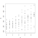
The source for my data is: https://vincentarelbundock.github.io/Rdatasets/csv/lme4/sleepstudy.csv
Plot()
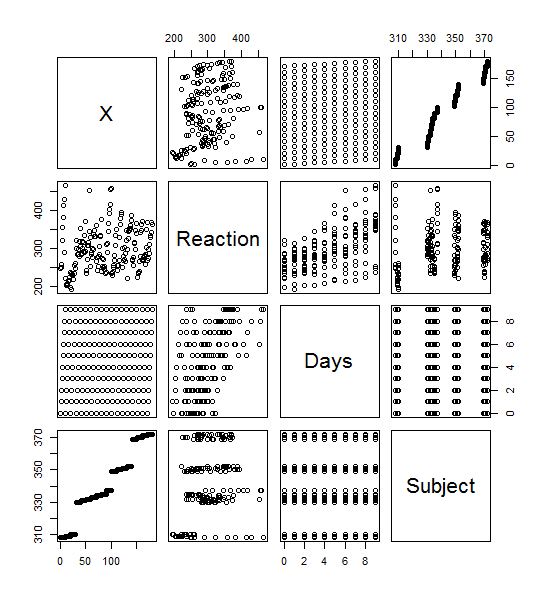
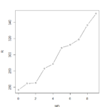
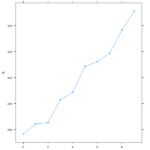
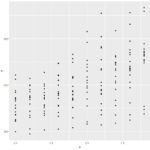
>plot(sleepstudy) yielded this lovely menagerie of graphs. it looks like it took all the variables and compared them to each other variable and made a metagraph. For example, you can look at square 3,3 and see that it compares the number of days going without sleep to the reaction time. Assigning the Days (D) and Reaction (R) to their own objects allows us to do plot(D,R) to get a larger version of that graph. Using the aggregate function, you can calculate the mean of each reaction measurement per day, assign them to objects, and plot them (>plot(MD,R, type=”b”).
Lattice()
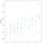
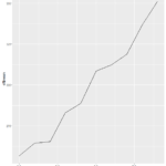
Similar graphs to the plot() graphs can be achieved with Latttice(). A simple >xyplot(Reaction~Days, sleepstudy) will yield the scatterplot below, and >xyplot(R~D, type=”b”) gives the line chart. The lattice graph is much more pleasing to look at. Having the y intervals oriented horizontally, having the intervals for the x and y values on both sides of the graph, and overall spacing give a much nicer look to the graph. Also, it’s utilization of the space in the frame is much better compared to the plot() graph, which looks like it has large, empty reserved space for a graph title.
ggplot2()
Ggplot2() adds a layer of complexity that is the idea of layers themselves. The bare bones “give me a graph quickly” plots from ggplot give graphs that are nicer than plot(). You get grid laid down across your graphs, with horizontal interval markers on the y axis. You also get even better space utilization than the quick-and-dirty lattice() graphs. The downside to the ggplot2() graphs is that the x intervals are less relatable. It defaulted to 2.5 day intervals for this particular graph, which makes analyzing the data significantly more abstract than full day or every-other-day intervals.
by Ryan | Mar 7, 2016 | intro to r programming
First, I made a new subset for the females from the original data, Dataset, and named it “females”.
>females <- subset(Dataset, Sex == “Female”)
I made a new object, ag, and used ddply to take the subset “Sex” from the object “females” and appended on the average grade by declaring transform as an argument. Ddply is part of the plyr package and follows a convenient naming convention that dictates the input and output data types. The first two letters determine if the respective input and outputs are an array, list, or data frame. They can also consist of multiple inputs or no inputs.
ag = ddply(females, “Sex”, transform, Average.Grade=mean(Grade))
Next, I saved a file of the data with the write function. Notably, it saves to your default directory for documents, and without a file extension added onto it. Using the argument sep=”,” will make the file a CSV file, which I found neat since CSV stands for comma separated values.
write.table(ag, “Sorted_average”, sep=”,”)
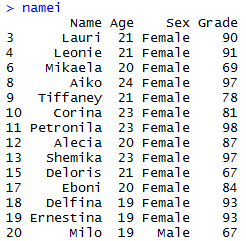
I made a new subset, namei, of the original dataset and used the grep() function to add the values from the column “Name”. Adding an “l” onto grep makes defines each value for the vector as either a match or mismatch (logical).
namei <- subset(Dataset, grepl(“[iI]”, Dataset$Name))
Finally, we can recall namei to see the printout of the table of all those i-named folk.
by Ryan | Feb 29, 2016 | intro to r programming
How do you tell what object system (S3 vs. S4) an object is associated with?
To determine what system an object uses, you are able to use a process of elimination with these commands.
is.object(x) – will return true if the thing you are testing is an object.
> is.object(Inventory_520782772_2016.February.07truncated)
[1] TRUE
isS4(object) – will return true if the object is an S4 object and false if it’s an S3 object.
> isS4(Inventory_520782772_2016.February.07truncated)
[1] FALSE
is(object , “refClass”) – will return true if your object is a reference class.
> is(Inventory_520782772_2016.February.07truncated, “refClass”)
[1] FALSE
How do you determine the base type (like integer or list) of an object?
In order to determine what the base type of an object is, you can use the command typeof() and it’ll return the object type
> typeof(Inventory_520782772_2016.February.07truncated)
[1] “list”
What is a generic function?
A generic function determines what method to call from the input it’s given. A S3 generic can take one argument, but a S4 generic can take multiple arguments.
What are the main differences between S3 and S4?
S3 systems are used the vast majority of the time and are simpler, less formal systems. S4 systems are more complicated, adding more formality to the syntax. S4 has the ability to use method dispatch to pass multiple arguments to a generic function and supports multiple inheritance, allowing you to inherit characteristics from multiple classes.
by Ryan | Feb 22, 2016 | intro to r programming
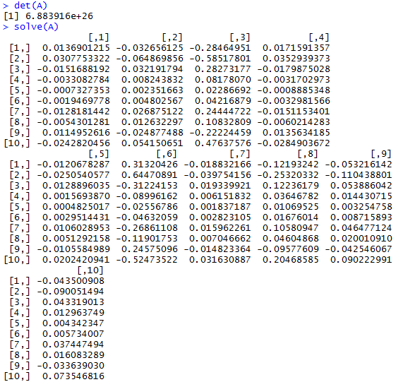
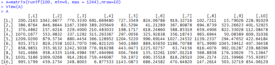
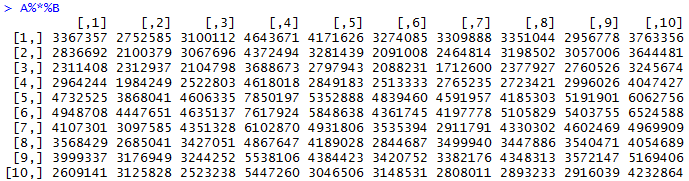
First, I created matrix A by randomly generating 100 numbers with the values between 0 and 100 and with 10 rows to make it square. It’s been ages since I’ve dealt with matrices, so I had to refamiliarize myself with how basic math functions work with them.
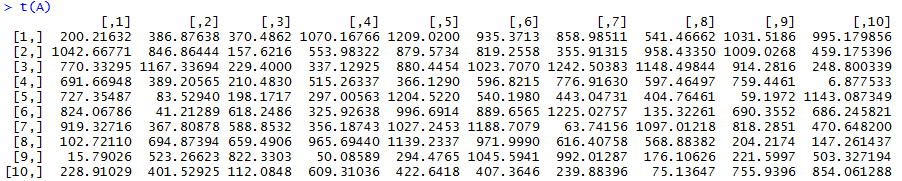
The transpose of A flips the values across the diagonal that connects [1,1] to [10,10] and is easily made with 4 short character strokes:
Next, I tried to create a randomized vector with > a=c(runif(10, min=0, max = 1244),nrow=10), but it ended up not working out, so I just made a numerically sequential vector with >a = c(1:10) to multiply with A. Each row of elements in the matrix are multiplied by the corresponding row in the vector.
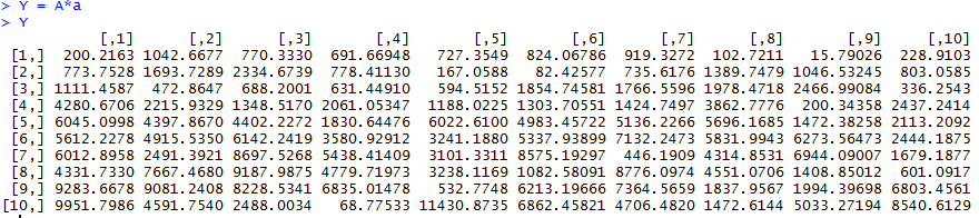
I multiplied matrix A with matrix B, which was made in the same randomized manner as matrix A:
We test the determinate of A to make sure it is inverseable and, in turn, solvable. > det(A) gives us a non-zero value, which gives us a green light to run > solve(A) and find the inverse of A.