by Ryan | Oct 31, 2016 | advanced statistics
> high <- c(10,9,8,9,10,8))
> moderate <- c(8,10,6,7,8,8)
> low <- c(4,6,6,4,2,2)
> reaction <- c(10,9,8,9,10,8,8,10,6,7,8,8,4,6,6,4,2,2)
> stresslvls <- c(rep("high",6), rep("moderate",6), rep("low",6))
> dat <- data.frame(reaction,stresslvls)
> analysis <- lm(reaction ~ as.factor(stresslvls), data = dat)
> anova(analysis)
Analysis of Variance Table

Response: stress
                      Df Sum Sq Mean Sq  F value     Pr(>F)
as.factor(stresslvls)  2 82.111  41.056   21.358  4.082e-05 ***
Residuals             15 28.833   1.922
---
Signif. codes: 0 ‘***’ 0.001 ‘**’ 0.01 ‘*’ 0.05 ‘.’ 0.1 ‘ ’ 1
The ANOVA test essentially breaks a sample down into smaller groups and compares the variance between the means of each of those groups to determine how much variance can be attributed to chance.
Here, we have analyzed a grouping of the reaction times of participants that were subjected to various levels of stress. Above, we can see the return of the ANOVA test. We can see that the between-group mean sum of squares is 41.056. This shows that the difference between each of the individual sample means and the mean of all the samples. The F value is the ratio between the mean squares of the mean squares. The larger the F statistic is, the more you can rule out the difference between the means being due to chance. The fact that the P value is so small allows us to reject the null hypothesis and claim that the level of stress the participants are subjected does have an effect on their reaction times.
by Ryan | Oct 24, 2016 | advanced statistics
- The mean for males is 3.571429 and the mean for females is 7.6
- The degrees of freedom for the t.test is 6.7687
- The T statistic is 2.8651
- The P value is 0.02505
- Yes
- +- 2.576
by Ryan | Oct 16, 2016 | advanced statistics
1a. H0: A cookie will break at more than 70 pounds of force or greater; u >= 70
Ha: A cookie will break at less than 70 pounds of force on average; u < 70
1b. yes
1c. p = 0.0359 There’s a 3.59% chance of finding a sample mean of 69.1 if u >=70.
1d. p = 0.0002 since p < 0.5, there is enough evidence to dismiss H0
1e. p = 0.0227 since p < 0.5, there is enough evidence to dismiss H0
2a. cor(mod8$Cost.per.serving, mod8$Fibber.per.serving)
2b. .228
2c: 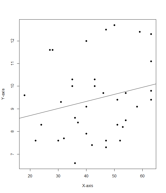
by Ryan | Oct 9, 2016 | advanced statistics
Q1. I created a function to do the calculations to find mu for the Confidence Interval:
ci <- function(xbar, con, sig, n)
{
con1 = con + ((1-con)/2)
mu = xbar + (qnorm(con1) * (sig / sqrt(n)))
sn = xbar – (qnorm(con1) * (sig / sqrt(n)))
paste(“The confidence interval is between “, sn, ” and “, +mu, ” and the estimated mean is “, xbar, sep =””)
}
The confidence intervals came in as follows:
> ci(115, .9, 15, 100)
[1] “The confidence interval is between 112.532719559573 and 117.467280440427 and the estimated mean is 115”
> ci(115, .95, 15, 100)
[1] “The confidence interval is between 112.06005402319 and 117.93994597681 and the estimated mean is 115”
> ci(115, .98, 15, 100)
[1] “The confidence interval is between 111.510478188939 and 118.489521811061 and the estimated mean is 115”
Q2
[1] “The confidence interval is between 83.0400360154599 and 86.9599639845401 and the estimated mean is 85”
Q3
((1.96 * 15) / 5)^2
[1] 34.5744
I think the minimum sample size should be 35 if I’m thinking of the zscore tails properly.
edit: After reviewing the last question, 35 is right, but how i got to it was wrong
III
The biggest thing to note about this is the difference between the 95% confidence interval and the 97.5th percentile ranking. Each tail of the 95% confidence interval contains 2.5% of the area under the curve. But we’re only looking for a single tailed value, so we must use qnorm(.975).
I feel like I was perhaps a little bit confused about what questions 1 and 2 were asking for, or what the answer should look like.
by Ryan | Oct 2, 2016 | advanced statistics
A
Import vector of values of ice cream purchase numbers
>a <- c(8, 14, 16, 10, 11)
Generate random sample of 2 values and save to a vector
> b <- sample(a,2)
[1] 10 11
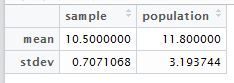
Calculate mean and standard deviation of the sample.
>mean(b)
[1] 10.5
> sd(b)
[1] 0.7071068
Create data.frame out of mean and stdev for the sample and population.
mean(a)
[1] 11.8
> sd(a)
[1] 3.193744
smp <- c(10.5,0.7071068)
> pop <- c(11.8,3.193744)
> c <- data.frame < (smp, pop)
B
- I think that the sample proportion will have the approximately the same distribution since nq = 5.
- I think 100 is the smallest value of n for which p is approximately normal because anything smaller than n = 100 will make np < 5. The high value of p is very limiting.