by Ryan | Feb 29, 2016 | intro to r programming
How do you tell what object system (S3 vs. S4) an object is associated with?
To determine what system an object uses, you are able to use a process of elimination with these commands.
is.object(x) – will return true if the thing you are testing is an object.
> is.object(Inventory_520782772_2016.February.07truncated)
[1] TRUE
isS4(object) – will return true if the object is an S4 object and false if it’s an S3 object.
> isS4(Inventory_520782772_2016.February.07truncated)
[1] FALSE
is(object , “refClass”) – will return true if your object is a reference class.
> is(Inventory_520782772_2016.February.07truncated, “refClass”)
[1] FALSE
How do you determine the base type (like integer or list) of an object?
In order to determine what the base type of an object is, you can use the command typeof() and it’ll return the object type
> typeof(Inventory_520782772_2016.February.07truncated)
[1] “list”
What is a generic function?
A generic function determines what method to call from the input it’s given. A S3 generic can take one argument, but a S4 generic can take multiple arguments.
What are the main differences between S3 and S4?
S3 systems are used the vast majority of the time and are simpler, less formal systems. S4 systems are more complicated, adding more formality to the syntax. S4 has the ability to use method dispatch to pass multiple arguments to a generic function and supports multiple inheritance, allowing you to inherit characteristics from multiple classes.
by Ryan | Feb 22, 2016 | intro to r programming
First, I created matrix A by randomly generating 100 numbers with the values between 0 and 100 and with 10 rows to make it square. It’s been ages since I’ve dealt with matrices, so I had to refamiliarize myself with how basic math functions work with them.

The transpose of A flips the values across the diagonal that connects [1,1] to [10,10] and is easily made with 4 short character strokes:

Next, I tried to create a randomized vector with > a=c(runif(10, min=0, max = 1244),nrow=10), but it ended up not working out, so I just made a numerically sequential vector with >a = c(1:10) to multiply with A. Each row of elements in the matrix are multiplied by the corresponding row in the vector.

I multiplied matrix A with matrix B, which was made in the same randomized manner as matrix A:

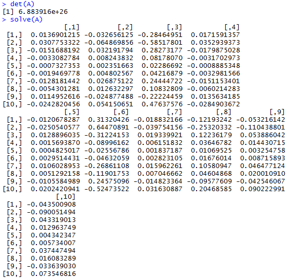
We test the determinate of A to make sure it is inverseable and, in turn, solvable. > det(A) gives us a non-zero value, which gives us a green light to run > solve(A) and find the inverse of A.

by Ryan | Feb 22, 2016 | intro to r programming
Here’s our starting data:
>Frequency_of_Visits<-c(0.6,0.3,0.4,0.4,0.2,0.6,0.3,0.4,0.9,0.2)
> Blood_Pressure<-c(103,87,32,42,59,109,78,205,135,176)
> First_Assessment<-c(1,1,1,1,0,0,0,0,NA,1)
> Second_Assessment<-c(0,0,1,1,0,0,1,1,1,1)
> Final_Decision<-c(0,1,0,1,0,1,0,1,1,1)
The values are the frequency of each patients’ doctor visits, their blood pressure measurements, first assessment (made by a general doctor), a second assessment (made by an external doctor), and a final decision (made by the head of the emergency unit). With all that loaded into the values, we move onto making some box and whisker plots and histograms. The real, unspoken, champ of this exercise is going to be:
par(mfrow=c(1,3))
This command lets us make a matrix with 1 row and 3 columns to which we will put our boxplots.
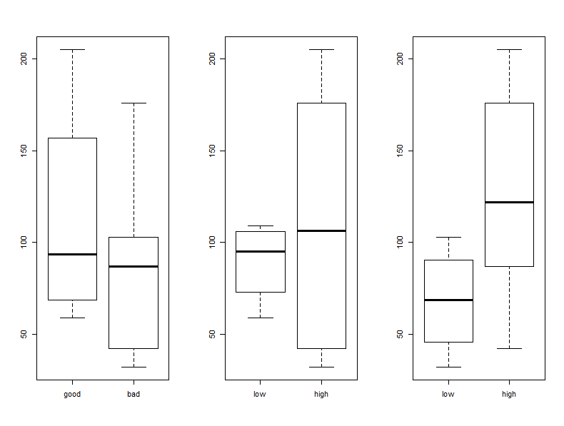
> boxplot(Blood_Pressure~First_Assessment, names=c(“good”,”bad”))
> boxplot(Blood_Pressure~Second_Assessment, names=c(“low”,”high”))
> boxplot(Blood_Pressure~Final_Decision, names=c(“low”,”high”))

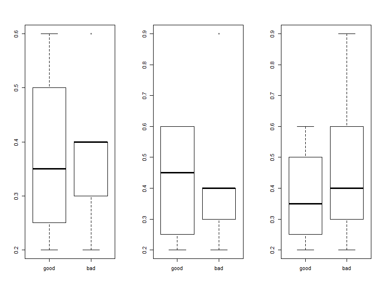
Here, we should note that “good” blood pressure is also “low priority”. The external doctor (plot 2) has a huge range in which they declare blood pressures to be high priority, and the general doctor seems to mostly consider relatively low values of blood pressure to be dangerous. Next up we’re going to compare the frequency of patients’ visits compared with the status of their blood pressure and we’ll see that first two doctors seem to note that people that visit less often are somewhat in more need of care.
> boxplot(Frequency_of_Visits~First_Assessment, names=c(“good”,”bad”))
> boxplot(Frequency_of_Visits~Second_Assessment, names=c(“good”,”bad”))
> boxplot(Frequency_of_Visits~Final_Decision, names=c(“good”,”bad”))

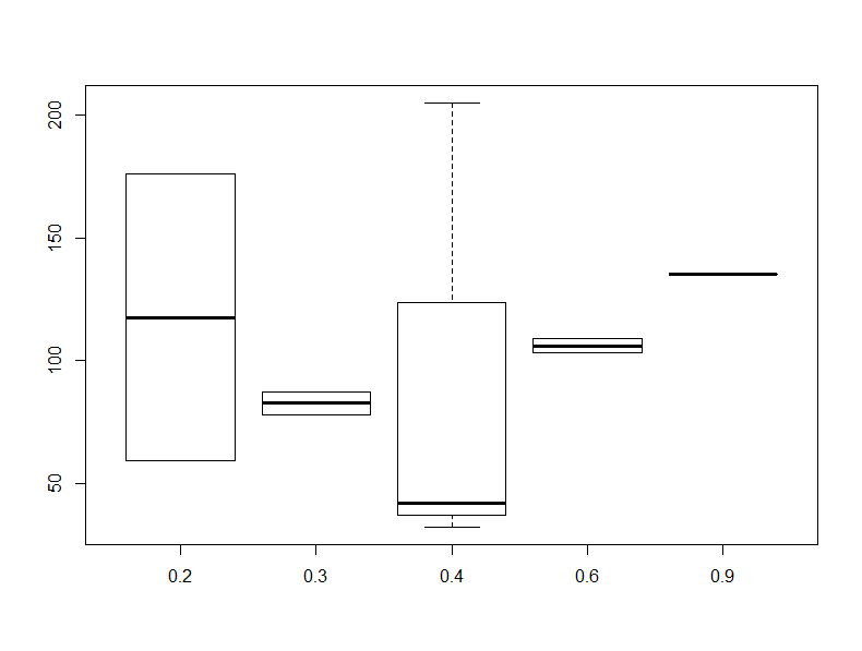
In order to make this next plot I had to reset my to be one row and column with par(mfrow=c(1,1)). This one will compare blood pressure to the frequency of visits and shows that the results are all over the board and that there’s really not that much data to make a good correlation anyways.
> par(mfrow=c(1,1))
> boxplot(Blood_Pressure~Frequency_of_Visits)

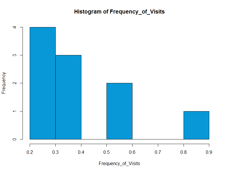
Finally, we make a histogram of the Frequency of visits, which shows that people are more likely to make less frequent visits.
> hist(Frequency_of_Visits, col=”#0898d7″)

by Ryan | Feb 8, 2016 | intro to r programming
Functions are great. You type up a little code, execute your function, and then watch as your automation takes over the world. Easy enough, right? Wrong. Well, sort of wrong. If you know what you want to do and how to do it, then it’s easy. If you know what you want to do, but don’t know how to do it, then it’s a little hard. And if you don’t know what you want to do (and probably wouldn’t now how to do it even if you did), then it’s hard. Luckily for me, I have a big fat database of Magic the Gathering cards I own and thought it’d be interesting to try to make a function on it. The easiest thing that i thought I could do would be various analyses on the casting cost of each card.

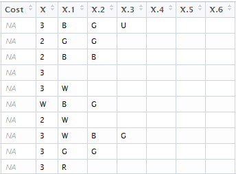
Knowing what I want to do? Check. The problem for me, though was how my database stored the information. Normally a card has some numbers and symbols showing how much it costs to play, and that cost can be converted to alphanumerical representation. For example, the card on the left has a cost of 6RR. For whatever reason, my database would have displayed that as {6}{R}{R}, which I suppose would be usable if I really knew what I was doing. But I don’t. I tried Googling around for how to split columns, but decided that that was over my head. So I cheated and went into Excel to quickly separate out the values into additional columns, then imported my new data back into R Studio. I used the count function to

Ugly “I don’t know what to do with these” Costs

Less Ugly “I can probably manage these” Costs
Make tables of each column and to give a, well, count of each value. From there I figured that I’d need to combine all 7 tables into one, but they had different column headers so I figured that I’d have to find out how to fix that too. I thought that that may take me a while, so I decided to just get started with my function and have it create all of the tables and figure out how to merge them together later. Well creating the function as essentially a batch command processor turned out to not be as straight forward as anticipated. I kept having the function try to call the series of
x <- count(Inventory_520782772_2016.February.07truncated, “X”)…
to make all of the tables from calling just my manasymbols function. Well that didn’t work. I tried making the tables as a data.frame and as.data.frame. I tried making the function with manasymbols <- function, manasymbols <- function(), and manasymbols <- function(x). After a long struggle of trying different combinations of these, I learned 1. that copy/pasting my code into R Studio doesn’t quite make the function properly and 2. that the function won’t make the object a global with just the x <-. I had to use x <<- in order for the object to be passed from inside of the function to the global level.
by Ryan | Feb 1, 2016 | intro to r programming
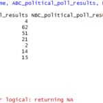
Warning message:
In mean.default(polls.df):
argument is not numerical or logical: returning NA
I hate this message. It has been the bane of me for far too long. From what I understand, this error gets thrown at you when the console tries to compute something that it can’t. In my case, the column for Name is not numeric.

I read that this is a relatively new problem, as R before version 3.0 would just ignore the illogical request. One way to get the right answer was with
colMeans(polls.df[,2:3])

and
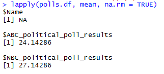
lapply(polls.df, mean, na.rm = TRUE)

Neither of these felt like particularly satisfactory ways to produce the mean. Through this process, I came up with some rather weird outputs that are useless. But I’m sure that looking back at these, from the future, will yield a good “What was I thinking?” moment, so I’ll include them.


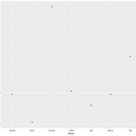
Getting ggplot working was a tough hike as well. I spent well over an hour trying to get a plot before I realized that, though I had installed the package, the library wasn’t loaded. Once I was able to get a basic plot working, I decided that I wanted to try to overlay both ABC_political_poll_results and NBC_political_poll_results onto one plot to show how the candidates vary between the two. But try as I might, I was not successful, so I have only two separate, basic graphs to show the candidate’s results for each respective poll.
ggplot(polls.df, aes(x = Name, y = _political_poll_results)) + geom_point() + geom_point(data = polls.df, aes(x = Name, y = _political_poll_results))
Unfortunately I wasn’t really able to get anything else constructive done, though I did just realize that summary() worked fine at calculating the means. That confuses me even more on why mean() wasn’t able to muster.

