by Ryan | Oct 9, 2016 | advanced statistics

Q1.  I created a function to do the calculations to find mu for the Confidence Interval:

ci <- function(xbar, con, sig, n)
{
con1 = con + ((1-con)/2)
mu = xbar + (qnorm(con1) * (sig / sqrt(n)))
sn = xbar – (qnorm(con1) * (sig / sqrt(n)))
paste(“The confidence interval is between “, sn, ” and “, +mu, ” and the estimated mean is “, xbar, sep =””)
}

The confidence intervals came in as follows:

> ci(115, .9, 15, 100)
[1] “The confidence interval is between 112.532719559573 and 117.467280440427 and the estimated mean is 115”
> ci(115, .95, 15, 100)
[1] “The confidence interval is between 112.06005402319 and 117.93994597681 and the estimated mean is 115”
> ci(115, .98, 15, 100)
[1] “The confidence interval is between 111.510478188939 and 118.489521811061 and the estimated mean is 115”

Q2

[1] “The confidence interval is between 83.0400360154599 and 86.9599639845401 and the estimated mean is 85”

Q3

((1.96 * 15) / 5)^2
[1] 34.5744

I think the minimum sample size should be 35 if I’m thinking of the zscore tails properly.

edit: After reviewing the last question, 35 is right, but how i got to it was wrong

III

The biggest thing to note about this is the difference between the 95% confidence interval and the 97.5th percentile ranking.  Each tail of the 95% confidence interval contains 2.5% of the area under the curve.  But we’re only looking for a single tailed value, so we must use qnorm(.975).

I feel like I was perhaps a little bit confused about what questions 1 and 2 were asking for, or what the answer should look like.

Sampling & Confidence interval Estimation

by Ryan | Oct 2, 2016 | advanced statistics

A

Import vector of values of ice cream purchase numbers

>a <- c(8, 14, 16, 10, 11)

Generate random sample of 2 values and save to a vector

> b <- sample(a,2)
[1] 10 11

Calculate mean and standard deviation of the sample.

>mean(b)
[1] 10.5
> sd(b)
[1] 0.7071068

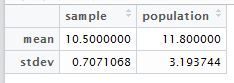
Create data.frame out of mean and stdev for the sample and population.

mean(a)
[1] 11.8
> sd(a)
[1] 3.193744

smp <- c(10.5,0.7071068)
> pop <- c(11.8,3.193744)
> c <- data.frame < (smp, pop)

B

1. I think that the sample proportion will have the approximately the same distribution since nq = 5.
2. I think 100 is the smallest value of n for which p is approximately normal because anything smaller than n = 100 will make np < 5.  The high value of p  is very limiting.

Bivariate Statistics

by Ryan | Sep 11, 2016 | advanced statistics

Initially, I was just going to calculate the correlation coefficient manually in R without using the functions, but then I decided that if I was going to do it manually then I may as well do it by hand.  I ended up making a mistake with spacing by not thinking about how many digits would be made out of squaring an already triple digit number.

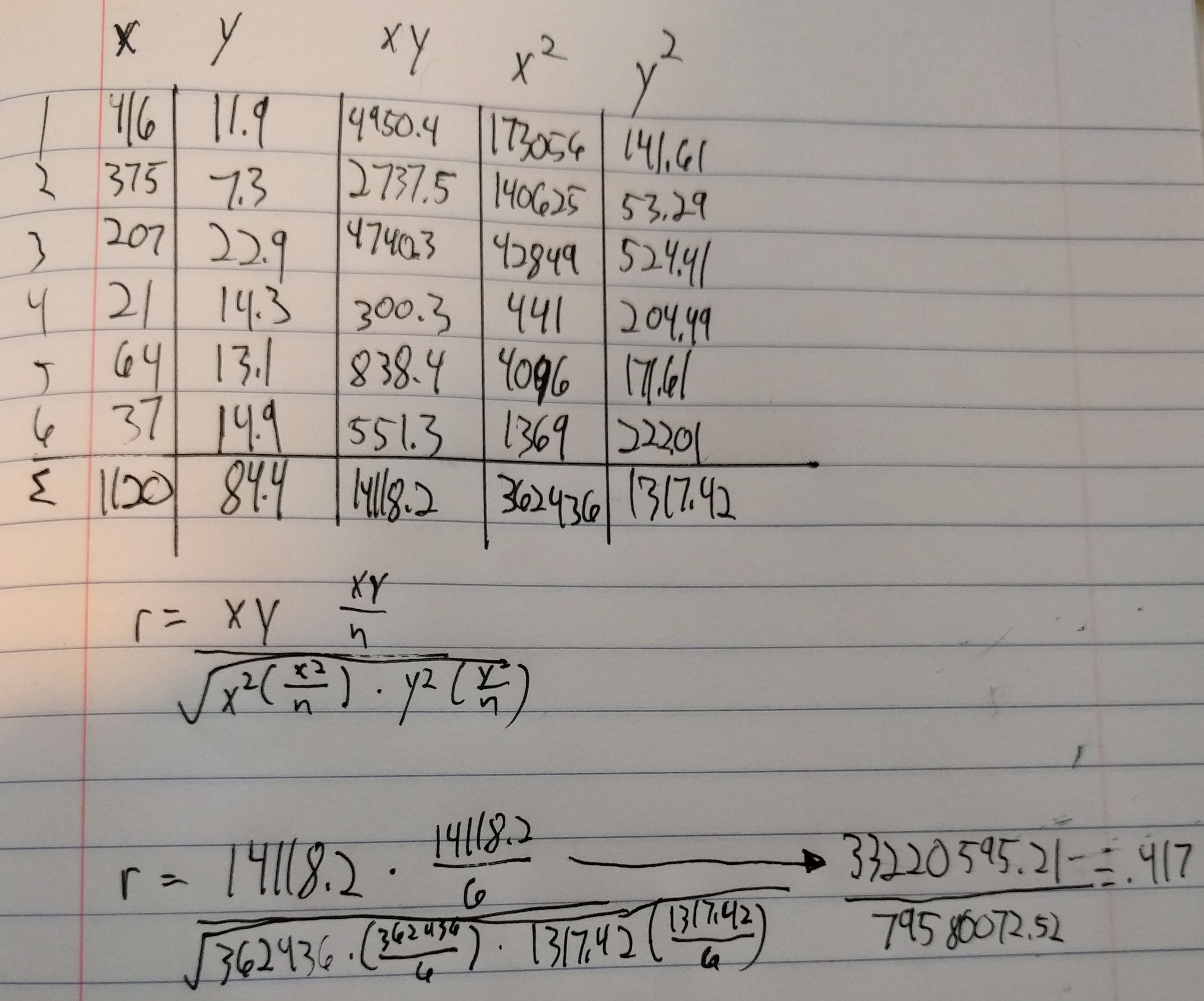
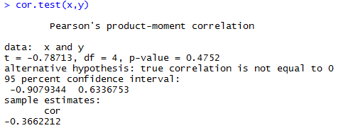
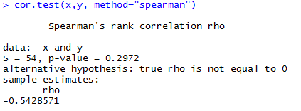
From there, inputting the x and y values into R and executing the cor.tests() were very simple and straightforward.  I feel like I’ve gotten to the point with R where I don’t feel like I’m completely lost all the time.

Module 2

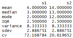
by Ryan | Sep 5, 2016 | advanced statistics

For this assignment, I decided to to make everything as one script and use the Source with Echo command to run it all at once.  The only issue I had is that mode() does not yield a mode.  It returns what storage mode the object uses, so I had to look up how to make a function to calculate the mode.

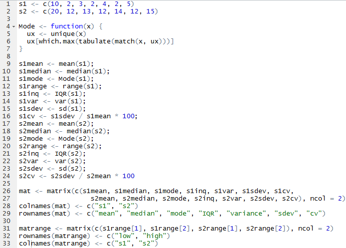
From there, I was able to call mat and matrange to pull up the tables of all the values.